Every formula has a sound. Hear it. Say it back. Watch it animate apart.
Touch the interactive widget. Type the code. No more bouncing off Greek letters.
Chapter 01 · 1 of 17
Vectors — arrows of numbers.
A vector is an ordered list of numbers. Stack them in a column, add other vectors to them, scale them by a single number. Foundation of everything.
click ANIMATE — Kokori will speak each step as it appears
ready
Pronunciation
Vector v equals, open bracket, v sub one, v sub two, dot dot dot, v sub n, close bracket. K vector v plus vector w, equals, component-wise sum.
SAY IT BACK · ELOCUTION
Vector v equals, open bracket, v sub one, v sub two, dot dot dot, v sub n, close bracket. K vector v plus vector w, equals, component-wise sum.
Tap Hear it first to listen, then Say it back. Speak naturally — we score how closely you match.
—
In plain English
A vector is a list of numbers, written as a column. Add two vectors by adding matching entries. Multiply a vector by a single number (a scalar) by multiplying every entry. Combining the two operations — k·v + w — is called a linear combination, and that single idea generates every other concept in linear algebra.
Symbol glossary — click any symbol to hear it
vvectoran ordered list of n numbers
vᵢi-th componentthe entry at position i
nndimension — number of components
kscalara single number (not a vector)
+vector additioncomponent-wise sum
Plug in a value — see each operation
🔢 Plug in a value · see every step
live arithmetic — type x and watch the formula compute
Interactive — touch it
v = [2.00, 1.00]w = [1.00, 2.00]k·v + w = [5.00, 4.00]
click ANIMATE — Kokori will speak each step as it appears
ready
Pronunciation
Norm of v equals, square root of, v sub one squared, plus v sub two squared, plus dot dot dot, plus v sub n squared.
SAY IT BACK · ELOCUTION
Norm of v equals, square root of, v sub one squared, plus v sub two squared, plus dot dot dot, plus v sub n squared.
Tap Hear it first to listen, then Say it back. Speak naturally — we score how closely you match.
—
In plain English
The norm (length, magnitude) of a vector is just Pythagoras in n dimensions. For v = [3, 4]: √(9 + 16) = √25 = 5. Sign doesn't matter — we square first. Output is always ≥ 0, and it's zero only when every component is zero.
Symbol glossary — click any symbol to hear it
‖v‖L2 normgeometric length of v
√square rootnon-negative root
Σsumadd everything that follows
vᵢ²squared componentalways non-negative
Plug in a value — see each operation
🔢 Plug in a value · see every step
live arithmetic — type x and watch the formula compute
click ANIMATE — Kokori will speak each step as it appears
ready
Pronunciation
v hat equals, v, divided by, norm of v.
SAY IT BACK · ELOCUTION
v hat equals, v, divided by, norm of v.
Tap Hear it first to listen, then Say it back. Speak naturally — we score how closely you match.
—
In plain English
A unit vector is a vector with length 1. To make one, just divide every component by the vector's own length. The hat — v̂ — is the universal notation for "normalized." Unit vectors strip the scale and let you compare pure directions, which is exactly what cosine similarity will do next.
click ANIMATE — Kokori will speak each step as it appears
ready
Pronunciation
a dot b equals, the sum from i equals one to n, of a sub i times b sub i. Same as, norm of a, times norm of b, times cosine theta.
SAY IT BACK · ELOCUTION
a dot b equals, the sum from i equals one to n, of a sub i times b sub i. Same as, norm of a, times norm of b, times cosine theta.
Tap Hear it first to listen, then Say it back. Speak naturally — we score how closely you match.
—
In plain English
The dot product has two equal definitions. Algebraically: multiply matching components, sum them. Geometrically: ‖a‖ · ‖b‖ · cos θ, where θ is the angle between a and b. Same number, two stories. Output is a SCALAR. Aligned vectors → big positive. Opposite → big negative. Perpendicular → exactly zero.
click ANIMATE — Kokori will speak each step as it appears
ready
Pronunciation
Cosine of theta equals, a dot b, divided by, norm of a times norm of b.
SAY IT BACK · ELOCUTION
Cosine of theta equals, a dot b, divided by, norm of a times norm of b.
Tap Hear it first to listen, then Say it back. Speak naturally — we score how closely you match.
—
In plain English
Take the dot product, then divide by the product of the lengths. The result is a number between −1 and 1. The magnitudes cancel — only the angle matters. This is why every embedding model (OpenAI, Anthropic, Cohere, Voyage) returns vectors you compare with cosine similarity: pure direction, scale-invariant.
click ANIMATE — Kokori will speak each step as it appears
ready
Pronunciation
A times x, sub i, equals, the sum from j equals one to n, of, A sub i j, times x sub j.
SAY IT BACK · ELOCUTION
A times x, sub i, equals, the sum from j equals one to n, of, A sub i j, times x sub j.
Tap Hear it first to listen, then Say it back. Speak naturally — we score how closely you match.
—
In plain English
A matrix A acts on a vector x and produces a new vector. The i-th entry of the output is the dot product of row i of A with x. Shapes: A is m×n, x is n×1, Ax is m×1. Every linear function from ℝⁿ to ℝᵐ can be written this way.
Symbol glossary — click any symbol to hear it
Amatrix Ashape m × n
Aᵢⱼentry i,jrow i, column j
xinput vectorshape n × 1
Axoutput vectorshape m × 1
Plug in a value — see each operation
🔢 Plug in a value · see every step
live arithmetic — type x and watch the formula compute
click ANIMATE — Kokori will speak each step as it appears
ready
Pronunciation
A B sub i j, equals, the sum from k equals one to n, of, A sub i k, times, B sub k j.
SAY IT BACK · ELOCUTION
A B sub i j, equals, the sum from k equals one to n, of, A sub i k, times, B sub k j.
Tap Hear it first to listen, then Say it back. Speak naturally — we score how closely you match.
—
In plain English
The (i, j) entry of AB is the dot product of A's i-th row and B's j-th column. Shapes: A is m×n, B is n×p, AB is m×p. The shared dimension n must match — otherwise the product is undefined. Conceptually, AB means "do B first, then A" — composition of transformations.
click ANIMATE — Kokori will speak each step as it appears
ready
Pronunciation
Determinant of a, b, c, d, equals, a times d, minus, b times c.
SAY IT BACK · ELOCUTION
Determinant of a, b, c, d, equals, a times d, minus, b times c.
Tap Hear it first to listen, then Say it back. Speak naturally — we score how closely you match.
—
In plain English
For a 2×2 matrix, the determinant is just ad − bc. Geometrically, this is the signed area of the parallelogram spanned by the matrix's columns. |det| tells you how much the matrix scales area; the sign tells you whether it flipped orientation. det = 0 means the matrix collapses 2D onto a line — it's singular and has no inverse.
Symbol glossary — click any symbol to hear it
detdeterminantsigned area scaling
admain diagonal producttop-left × bottom-right
bcanti-diagonal producttop-right × bottom-left
0zero determinantsingular — no inverse
Plug in a value — see each operation
🔢 Plug in a value · see every step
live arithmetic — type x and watch the formula compute
click ANIMATE — Kokori will speak each step as it appears
ready
Pronunciation
A times v equals, lambda times v. Lambda equals one half, trace of A, plus or minus, square root of, trace of A squared minus four det A.
SAY IT BACK · ELOCUTION
A times v equals, lambda times v. Lambda equals one half, trace of A, plus or minus, square root of, trace of A squared minus four det A.
Tap Hear it first to listen, then Say it back. Speak naturally — we score how closely you match.
—
In plain English
An eigenvector of a matrix A is a non-zero vector v that A merely stretches — Av = λv. The scalar λ is the eigenvalue. For any 2×2 matrix, eigenvalues solve the quadratic λ² − (trace)λ + det = 0. Trace = sum of diagonal entries. Det = ad − bc. Eigenpairs are the DNA of a matrix — PCA, PageRank, and Schrödinger's equation all reduce to "find the eigenpairs."
click ANIMATE — Kokori will speak each step as it appears
ready
Pronunciation
Sigma of x equals one over, one plus, e to the negative x.
SAY IT BACK · ELOCUTION
Sigma of x equals one over, one plus, e to the negative x.
Tap Hear it first to listen, then Say it back. Speak naturally — we score how closely you match.
—
In plain English
Read it as: σ of x means "apply the sigmoid function to x". Output is one divided by (one plus e to the negative x). Big positive x gives ~1. Big negative x gives ~0. Middle x=0 gives 0.5.
click ANIMATE — Kokori will speak each step as it appears
ready
Pronunciation
Rell-you of x equals, the maximum of zero and x.
SAY IT BACK · ELOCUTION
Rell-you of x equals, the maximum of zero and x.
Tap Hear it first to listen, then Say it back. Speak naturally — we score how closely you match.
—
In plain English
Read: "ReLU of x" is whichever is bigger — zero, or x itself. ReLU dominates modern networks because it is fast and the gradient is either 1 or 0 — clean backprop.
click ANIMATE — Kokori will speak each step as it appears
ready
Pronunciation
Softmax of z sub i, equals, e to the z sub i, divided by, the sum from j equals one to K, of e to the z sub j.
SAY IT BACK · ELOCUTION
Softmax of z sub i, equals, e to the z sub i, divided by, the sum from j equals one to K, of e to the z sub j.
Tap Hear it first to listen, then Say it back. Speak naturally — we score how closely you match.
—
In plain English
Read: softmax takes the i-th element of vector z, divides e to that element by the sum of e to all elements. Result: probability per class, all summing to 1. Σ means "add up everything that follows".
click ANIMATE — Kokori will speak each step as it appears
ready
Pronunciation
L equals, one over n, times the sum from i equals one to n, of, y sub i minus y-hat sub i, squared.
SAY IT BACK · ELOCUTION
L equals, one over n, times the sum from i equals one to n, of, y sub i minus y-hat sub i, squared.
Tap Hear it first to listen, then Say it back. Speak naturally — we score how closely you match.
—
In plain English
Read: loss L equals one over n times the sum, for every sample i from 1 to n, of (true minus predicted) squared. Squaring punishes big errors disproportionately.
click ANIMATE — Kokori will speak each step as it appears
ready
Pronunciation
L equals, negative the sum from i equals one to K, of, y sub i, times, log of y-hat sub i.
SAY IT BACK · ELOCUTION
L equals, negative the sum from i equals one to K, of, y sub i, times, log of y-hat sub i.
Tap Hear it first to listen, then Say it back. Speak naturally — we score how closely you match.
—
In plain English
Read: loss equals negative sum across all K classes of (true label) times log(predicted probability). Confident-correct gives tiny loss. Confident-wrong gives huge loss. The minus sign flips it positive.
click ANIMATE — Kokori will speak each step as it appears
ready
Pronunciation
Theta at time t plus one, equals, theta at time t, minus, eta times, the gradient with respect to theta, of L of theta at time t.
SAY IT BACK · ELOCUTION
Theta at time t plus one, equals, theta at time t, minus, eta times, the gradient with respect to theta, of L of theta at time t.
Tap Hear it first to listen, then Say it back. Speak naturally — we score how closely you match.
—
In plain English
Read: next weights (θ_t+1) equal current weights (θ_t) minus η times the gradient of loss with respect to weights. Gradient points UPHILL; subtracting moves DOWNHILL. Eta is the learning rate.
click ANIMATE — Kokori will speak each step as it appears
ready
Pronunciation
Partial L with respect to w, equals, partial L with respect to a, times, partial a with respect to z, times, partial z with respect to w.
SAY IT BACK · ELOCUTION
Partial L with respect to w, equals, partial L with respect to a, times, partial a with respect to z, times, partial z with respect to w.
Tap Hear it first to listen, then Say it back. Speak naturally — we score how closely you match.
—
In plain English
Read: derivative of loss with respect to a weight equals product of three derivatives along the path. Chain rule from calculus, run backwards through every layer. That is backpropagation.
click ANIMATE — Kokori will speak each step as it appears
ready
Pronunciation
Attention of Q, K, V, equals, softmax of, Q times K transpose, divided by, square root of d sub k, all times V.
SAY IT BACK · ELOCUTION
Attention of Q, K, V, equals, softmax of, Q times K transpose, divided by, square root of d sub k, all times V.
Tap Hear it first to listen, then Say it back. Speak naturally — we score how closely you match.
—
In plain English
Read: Q · K^T gets similarity scores. Divide by √d_k for stability. Softmax gives weights summing to 1. Multiply by V. Each token gets a weighted blend of all tokens' values.
Symbol glossary — click any symbol to hear it
QQ (queries)what each token is looking for
KK (keys)what each token offers
VV (values)the payload each token carries
KᵀK transposeK with rows and columns swapped
dₖd sub kdimension of key vectors
Plug in a value — see each operation
🔢 Plug in a value · see every step
live arithmetic — type x and watch the formula compute